Notebook example
An IPython (Jupyter) notebook showing this package usage is available at:
Script example
This example use randoms values for wind speed and direction(ws and wd variables). In situation, these variables are loaded with reals values (1-D array), from a database or directly from a text file (see the “load” facility from the matplotlib.pylab interface for that).
from windrose import WindroseAxes
from matplotlib import pyplot as plt
import matplotlib.cm as cm
import numpy as np

# Create wind speed and direction variables

ws = np.random.random(500) * 6
wd = np.random.random(500) * 360
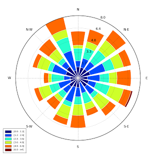
A stacked histogram with normed (displayed in percent) results
ax = WindroseAxes.from_ax()
ax.bar(wd, ws, normed=True, opening=0.8, edgecolor='white')
ax.set_legend()
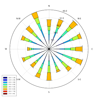
Another stacked histogram representation, not normed, with bins limits
ax = WindroseAxes.from_ax()
ax.box(wd, ws, bins=np.arange(0, 8, 1))
ax.set_legend()
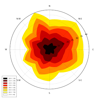
A windrose in filled representation, with a controlled colormap
ax = WindroseAxes.from_ax()
ax.contourf(wd, ws, bins=np.arange(0, 8, 1), cmap=cm.hot)
ax.set_legend()
Same as above, but with contours over each filled region…
ax = WindroseAxes.from_ax()
ax.contourf(wd, ws, bins=np.arange(0, 8, 1), cmap=cm.hot)
ax.contour(wd, ws, bins=np.arange(0, 8, 1), colors='black')
ax.set_legend()

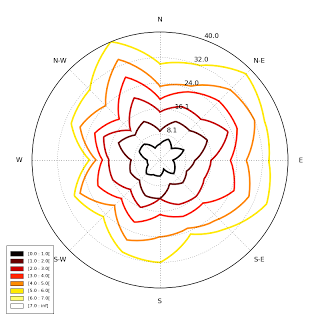
…or without filled regions
ax = WindroseAxes.from_ax()
ax.contour(wd, ws, bins=np.arange(0, 8, 1), cmap=cm.hot, lw=3)
ax.set_legend()
After that, you can have a look at the computed values used to plot the
windrose with the ax._info dictionary :
ax._info['bins']: list of bins (limits) used for wind speeds. If not set in the call, bins will be set to 6 parts between wind speed min and max.ax._info['dir']: list of directions “boundaries” used to compute the distribution by wind direction sector. This can be set by the nsector parameter (see below).ax._info['table']: the resulting table of the computation. It’s a 2D histogram, where each line represents a wind speed class, and each column represents a wind direction class.
So, to know the frequency of each wind direction, for all wind speeds, do:
ax.bar(wd, ws, normed=True, nsector=16)
table = ax._info['table']
wd_freq = np.sum(table, axis=0)
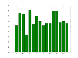
and to have a graphical representation of this result :
direction = ax._info['dir']
wd_freq = np.sum(table, axis=0)
plt.bar(np.arange(16), wd_freq, align='center')
xlabels = ('N','','N-E','','E','','S-E','','S','','S-O','','O','','N-O','')
xticks=arange(16)
gca().set_xticks(xticks)
draw()
gca().set_xticklabels(xlabels)
draw()
In addition of all the standard pyplot parameters, you can pass special
parameters to control the windrose production. For the stacked histogram
windrose, calling help(ax.bar) will give :
bar(self, direction, var, **kwargs) method of
windrose.WindroseAxes instance Plot a windrose in bar mode. For each
var bins and for each sector, a colored bar will be draw on the axes.
Mandatory:
direction: 1D array - directions the wind blows from, North centredvar: 1D array - values of the variable to compute. Typically the wind speeds
Optional:
nsector: integer - number of sectors used to compute the windrose table. If not set, nsectors=16, then each sector will be 360/16=22.5°, and the resulting computed table will be aligned with the cardinals points.bins: 1D array or integer - number of bins, or a sequence of bins variable. If not set, bins=6 between min(var) and max(var).blowto: bool. If True, the windrose will be pi rotated, to show where the wind blow to (useful for pollutant rose).colors: string or tuple - one string color ('k'or'black'), in this case all bins will be plotted in this color; a tuple of matplotlib color args (string, float, rgb, etc), different levels will be plotted in different colors in the order specified.cmap: a cm Colormap instance frommatplotlib.cm. - ifcmap == Noneandcolors == None, a default Colormap is used.edgecolor: string - The string color each edge bar will be plotted. Default : no edgecoloropening: float - between 0.0 and 1.0, to control the space between each sector (1.0 for no space)mean_values: Bool - specify wind speed statistics with direction=specific mean wind speeds. If this flag is specified, var is expected to be an array of mean wind speeds corresponding to each entry indirection. These are used to generate a distribution of wind speeds assuming the distribution is Weibull with shape factor = 2.weibull_factors: Bool - specify wind speed statistics with direction=specific weibull scale and shape factors. If this flag is specified, var is expected to be of the form [[7,2], …., [7.5,1.9]] where var[i][0] is the weibull scale factor and var[i][1] is the shape factor
probability density function (pdf) and fitting Weibull distribution
A probability density function can be plot using:
from windrose import WindAxes
ax = WindAxes.from_ax()
bins = np.arange(0, 6 + 1, 0.5)
bins = bins[1:]
ax, params = ax.pdf(ws, bins=bins)
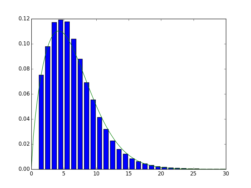
Optimal parameters of Weibull distribution can be displayed using
print(params)
(1, 1.7042156870194352, 0, 7.0907180300605459)
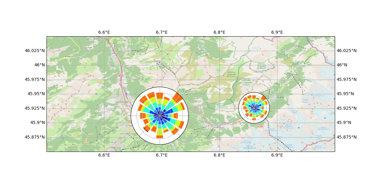
Overlay of a map
This example illustrate how to set an windrose axe on top of any other axes. Specifically, overlaying a map is often useful. It rely on matplotlib toolbox inset_axes utilities.
import numpy as np
import matplotlib.pyplot as plt
from mpl_toolkits.axes_grid.inset_locator import inset_axes
import cartopy.crs as ccrs
import cartopy.io.img_tiles as cimgt

import windrose

ws = np.random.random(500) * 6
wd = np.random.random(500) * 360

minlon, maxlon, minlat, maxlat = (6.5, 7.0, 45.85, 46.05)

proj = ccrs.PlateCarree()
fig = plt.figure(figsize=(12, 6))
# Draw main ax on top of which we will add windroses
main_ax = fig.add_subplot(1, 1, 1, projection=proj)
main_ax.set_extent([minlon, maxlon, minlat, maxlat], crs=proj)
main_ax.gridlines(draw_labels=True)
main_ax.coastlines()

request = cimgt.OSM()
main_ax.add_image(request, 12)

# Coordinates of the station we were measuring windspeed
cham_lon, cham_lat = (6.8599, 45.9259)
passy_lon, passy_lat = (6.7, 45.9159)

# Inset axe it with a fixed size
wrax_cham = inset_axes(main_ax,
        width=1,                             # size in inches
        height=1,                            # size in inches
        loc='center',                        # center bbox at given position
        bbox_to_anchor=(cham_lon, cham_lat), # position of the axe
        bbox_transform=main_ax.transData,    # use data coordinate (not axe coordinate)
        axes_class=windrose.WindroseAxes,    # specify the class of the axe
        )

# Inset axe with size relative to main axe
height_deg = 0.1
wrax_passy = inset_axes(main_ax,
        width="100%",                        # size in % of bbox
        height="100%",                       # size in % of bbox
        #loc='center',  # don't know why, but this doesn't work.
        # specify the center lon and lat of the plot, and size in degree
        bbox_to_anchor=(passy_lon-height_deg/2, passy_lat-height_deg/2, height_deg, height_deg),
        bbox_transform=main_ax.transData,
        axes_class=windrose.WindroseAxes,
        )

wrax_cham.bar(wd, ws)
wrax_passy.bar(wd, ws)
for ax in [wrax_cham, wrax_passy]:
  ax.tick_params(labelleft=False, labelbottom=False)
Functional API
Instead of using object oriented approach like previously shown, some
“shortcut” functions have been defined: wrbox, wrbar,
wrcontour, wrcontourf, wrpdf. See unit
tests.
Pandas support
windrose not only supports Numpy arrays. It also supports also Pandas
DataFrame. plot_windrose function provides most of plotting features
previously shown.
from windrose import plot_windrose
N = 500
ws = np.random.random(N) * 6
wd = np.random.random(N) * 360
df = pd.DataFrame({'speed': ws, 'direction': wd})
plot_windrose(df, kind='contour', bins=np.arange(0.01,8,1), cmap=cm.hot, lw=3)
Mandatory:
df: Pandas DataFrame withDateTimeIndexas index and at least 2 columns ('speed'and'direction').
Optional:
kind: kind of plot (might be either,'contour','contourf','bar','box','pdf')var_name: name of var column name ; default value isVAR_DEFAULT='speed'direction_name: name of direction column name ; default value isDIR_DEFAULT='direction'clean_flag: cleanup data flag (remove data points withNaN,var=0) before plotting ; default value isTrue.
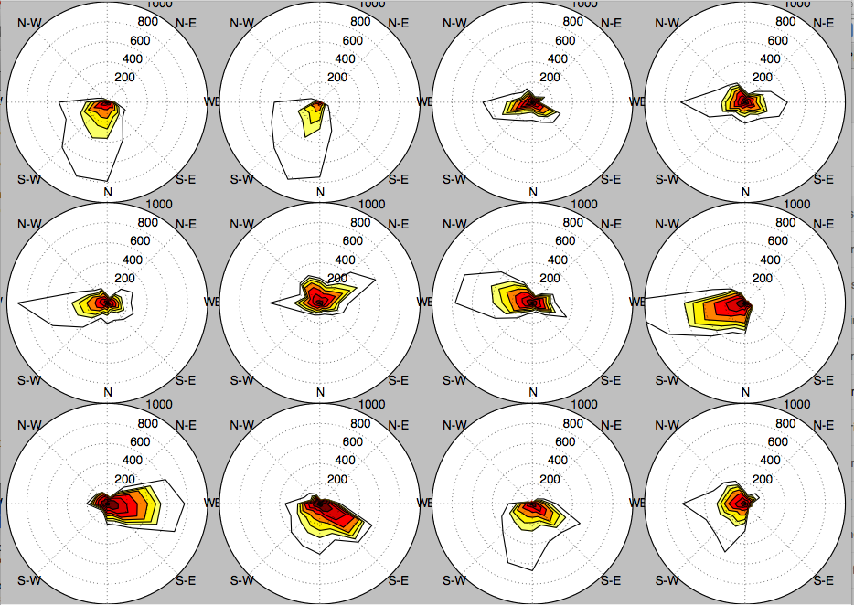
Subplots
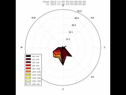
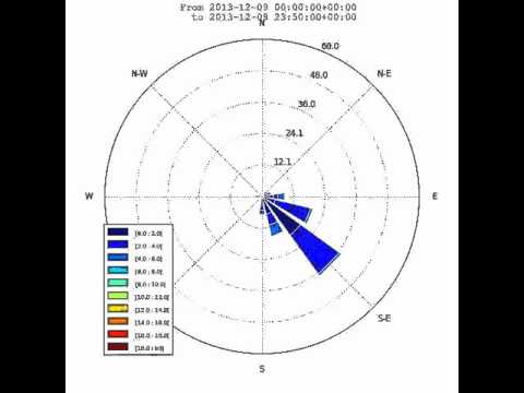
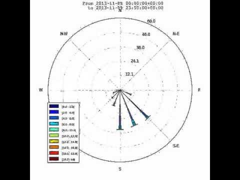
Video export
A video of plots can be exported. A playlist of videos is available at https://www.youtube.com/playlist?list=PLE9hIvV5BUzsQ4EPBDnJucgmmZ85D_b-W
See:
This is just a sample for now. API for video need to be created.
Use:
$ python samples/example_animate.py --help
to display command line interface usage.